Ordered dithering is an algorithm for adding noise to images with reduced color palette. Dithering can be applied to the final image as a post processing effect and does not change its looks in any particular way while fixing most precision related issues in the darkest areas of the image. All this effect does is it adds slight noise to color gradients so the human eye can perceive more colors than there really are.

High Definition Image

Naively Reduced Color Depth

Color Depth Reduced Through Dithering

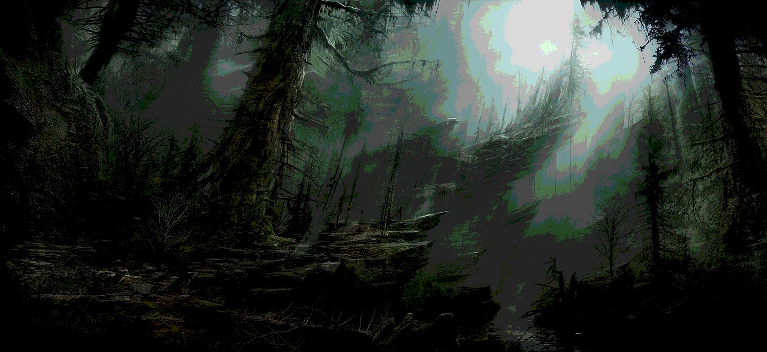
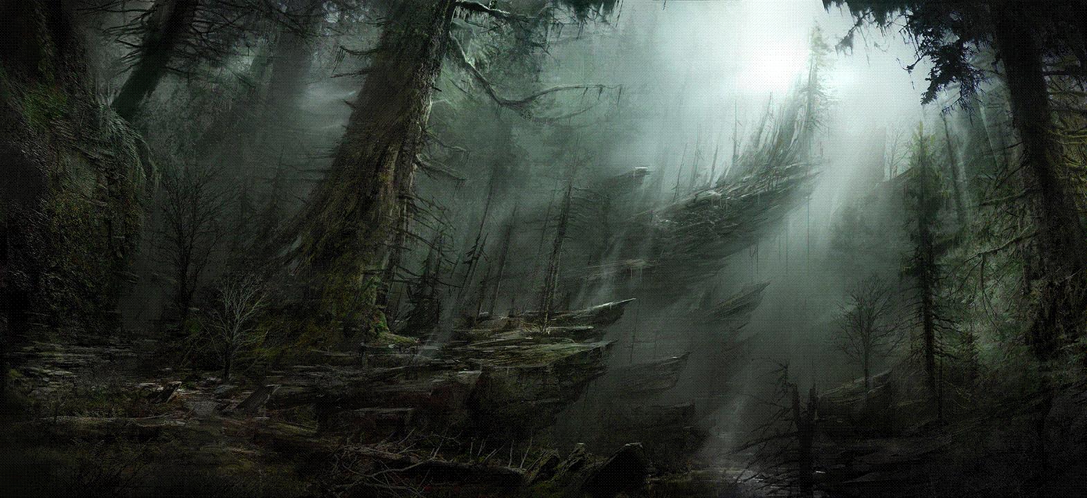
As you can see, in such detailed images dithering result is almost indistinguishable from the original image while naive color depth reduction resulted in some awful banding in the moonlight glimmer. Color depth in above example was reduced from 8 bits down to just 3, so dithering can also be used to compress pictures and this technique is indeed very often used to reduce size of GIFs.

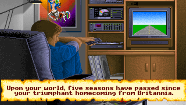
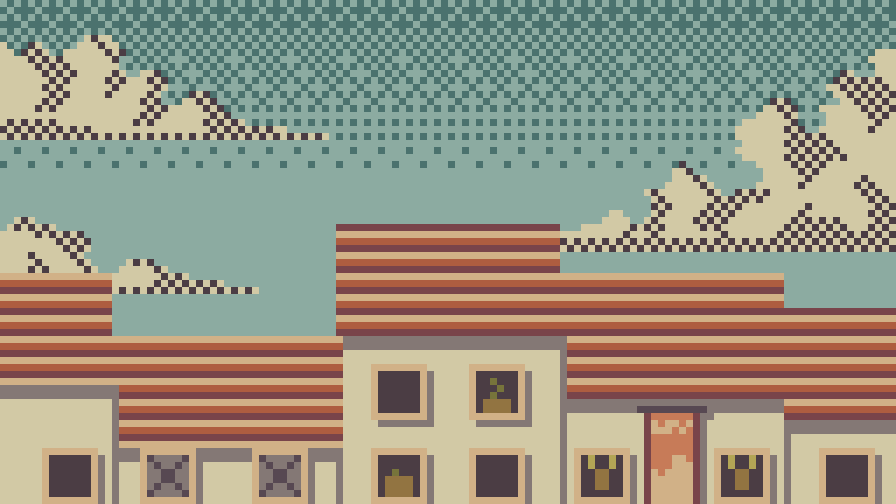
Ordered dithering is a technique pariticularly known for its broad use in the past when low color depth displays were commonly in use. It allowed human eye to perceive more colors than a screen was really able to support. It might not be obvious at first, but dithering is still commonly used even today in high fidelity computer graphics to reduce banding and low-precision artifacts, which turn out to appear even with the modern 8-bit displays. Ordered dithering is also a great way to obtain specific aesthetic in pixel art.

Dithering in Ultima VI: The False Prophet

Dithering in Pixel Art

The algorithm uses a tiled threshold matrix to decide whether to pick the closest quantized value from below or above the precise value we need to represent. Said matrix was developed by Bryce Bayer in 1973 and thus is called the "Bayer matrix".

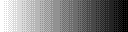
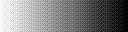
Here are Bayer matrices of three common sizes tiled over a 32x32 area:

2x2

4x4

8x8

You can observe that larger sizes of the matrix have a more randomized pattern. This allows dithering to represent more fictional colors, but over a wider area.

For your convenience, I include the above matrices in the form of a GLSL snippet:

const float[2][2] bayer2X2 = float[2][2](
	float[4](0.0 / 4.0, 3.0 / 4.0),
	float[4](2.0 / 4.0, 1.0 / 4.0)
);

const float[4][4] bayer4X4 = float[4][4](
	float[4]( 0.0 / 16.0, 12.0 / 16.0,  3.0 / 16.0, 15.0 / 16.0),
	float[4]( 8.0 / 16.0,  4.0 / 16.0, 11.0 / 16.0,  7.0 / 16.0),
	float[4]( 2.0 / 16.0, 14.0 / 16.0,  1.0 / 16.0, 13.0 / 16.0),
	float[4](10.0 / 16.0,  6.0 / 16.0,  9.0 / 16.0,  5.0 / 16.0)
);

const float[8][8] bayer8X8 = float[8][8](
	float[8]( 0.0 / 64.0, 48.0 / 64.0, 12.0 / 64.0, 60.0 / 64.0,  3.0 / 64.0, 51.0 / 64.0, 15.0 / 64.0, 63.0 / 64.0),
	float[8](32.0 / 64.0, 16.0 / 64.0, 44.0 / 64.0, 28.0 / 64.0, 35.0 / 64.0, 19.0 / 64.0, 47.0 / 64.0, 31.0 / 64.0),
	float[8]( 8.0 / 64.0, 56.0 / 64.0,  4.0 / 64.0, 52.0 / 64.0, 11.0 / 64.0, 59.0 / 64.0,  7.0 / 64.0, 55.0 / 64.0),
	float[8](40.0 / 64.0, 24.0 / 64.0, 36.0 / 64.0, 20.0 / 64.0, 43.0 / 64.0, 27.0 / 64.0, 39.0 / 64.0, 23.0 / 64.0),
	float[8]( 2.0 / 64.0, 50.0 / 64.0, 14.0 / 64.0, 62.0 / 64.0,  1.0 / 64.0, 49.0 / 64.0, 13.0 / 64.0, 61.0 / 64.0),
	float[8](34.0 / 64.0, 18.0 / 64.0, 46.0 / 64.0, 30.0 / 64.0, 33.0 / 64.0, 17.0 / 64.0, 45.0 / 64.0, 29.0 / 64.0),
	float[8](10.0 / 64.0, 58.0 / 64.0,  6.0 / 64.0, 54.0 / 64.0,  9.0 / 64.0, 57.0 / 64.0,  5.0 / 64.0, 53.0 / 64.0),
	float[8](42.0 / 64.0, 26.0 / 64.0, 38.0 / 64.0, 22.0 / 64.0, 41.0 / 64.0, 25.0 / 64.0, 37.0 / 64.0, 21.0 / 64.0)
);

Explaining stuff is usually best done with code, so let's get right in to it! Below you can see an exemplary implementation of ordered dithering:

float dither4X4(in float value, in ivec2 pixelPos, in int quantizedMax) {
	value *= float(quantizedMax);
	float floorValue = floor(value);
	
	float delta = value - floorValue;
	float edge = bayer4X4[pixelPos.x % 4][pixelPos.y % 4];
	
	return (floorValue + step(edge, delta)) / float(quantizedMax);
}

The short description of the above routine is that it returns a quantized value determined by the tiled bayer matrix' value at pixel's position. At first glance this explanation might be difficult to make sense of, so I will break it down for easy digestion.

First of all, what does quantized even mean? Wikipedia defines qunatization as "the process of constraining an input from a continuous or otherwise large set of values (such as the real numbers) to a discrete set (such as the integers)." So it's really just a fancy word for limiting the number of distinct values a variable can have. In the world of computing everything is quantized. Particularly digital color values are always quantized because computers only use a limited amount of bits per value. So in your shaders with 32-bit floating point values this quantization is almost invisible, but while outputting to an 8-bit display, we're restricted to only 256 distinct values per color channel.

Smooth

Naively Quantized

The function accepts three parameters:

• The first parameter to this function is an in float value. This is the unconstrained 32-bit color we want the user to perceive. It must confine in the standard range [0, 1].
• Next, there is an in ivec2 pixelPos. The pixel position is needed here to select appropriate value from the Bayer matrix virtually tiled over the screen.
• The last parameter is quantizedMax. It's the number of quantized values we want to divide the mentioned 32-bit floating point [0, 1] range into, minus one. For an 8-bit display output one would set it to 2^8 - 1 = 255.

The first step is to obtain the closest quantized value available below the exact value, the float floorValue. Next we compute the distance of this quantized value from the original value. We also fetch float edge from the bayer matrix of choice. The final step is to choose a quantized value either from below or above the original input by comparing computed distance to the predefined edge-distance. The + step(...) trick in the code above can alternatively be written down using the ternary operator where floorValue + 1.0 is simply the next available quantized value after floorValue:

delta < edge ? floorValue : floorValue + 1.0

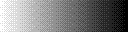
In the end we're left with quantized value for this current pixel. Below you can see the effect of this whole operation on the above white-to-black gradient. The results are restricted to the exact same palette of quantized values as the "Naively Quantized" version and the resolution is also smaller to make dithering more visible.

2x2 Bayer Matrix

4x4 Bayer Matrix

8x8 Bayer Matrix

For the matter of compression ordered dithering is simply a trade of color depth for resolution. It can create exceptionally cozy and rustical aesthetics in pixel art. And as for writing shaders, ordered dithering is a cheap operation and should almost always be used before writing to 8-bit output to maximize image quality. Dithering is applied after gamma-correction and directly before output because it quantizes color for the GPU to encode in a low precision format.

And that's all. Thanks for reading!

• Bryce Bayer - "An optimum method for two-level rendition of continuous-tone pictures"

All external images in this article are used solely for illustration and under fair use guidelines:

• "Dark forest environment" by Eric Gagnon @ Art Station
• Cutscene Photo from "Ultima VI: The False Prophet" by Origin Systems
• "Suburban Landscape" by u/kalamplee @ Reddit